CleanWatt

The problem

Ontario's residential electricity price is mostly regulated Time-of-Use — a fixed schedule, no model required. Carbon intensity is different: it swings dramatically as the grid shifts between near-zero-carbon nuclear, hydro, and wind and gas peakers. Running your dishwasher at 6pm vs. 11pm can mean a meaningful difference in emissions — but only if you know when the gas peakers fire. No consumer tool surfaces that.

What I built

An ingestion pipeline pulls hourly fuel-mix data from IESO's public XML reports via gridstatus, converts each hour's generation breakdown to gCO₂/kWh using standard per-fuel emission factors, and builds a validated hourly carbon-intensity series going back to 2023.

On top of that series I trained 24 independent LightGBM models — one per forecast horizon, t+1 through t+24. Direct multi-step forecasting: each model targets its own horizon directly rather than feeding predictions back into future steps, so errors don't compound. Features include calendar signals, carbon intensity lags, the current fuel mix breakdown, IESO's demand forecast, and Open-Meteo wind speed leads at 6h, 12h, and 24h.

A walk-forward backtest across 29 monthly expanding-window folds (2023-07 → 2026-06) evaluated the models honestly: train on all history before a cutoff, evaluate on the following month, never shuffle. Mean skill score across all 24 horizons: +0.301 vs. the "same hour yesterday" baseline. h=1 MAE is 4.98 gCO₂/kWh.

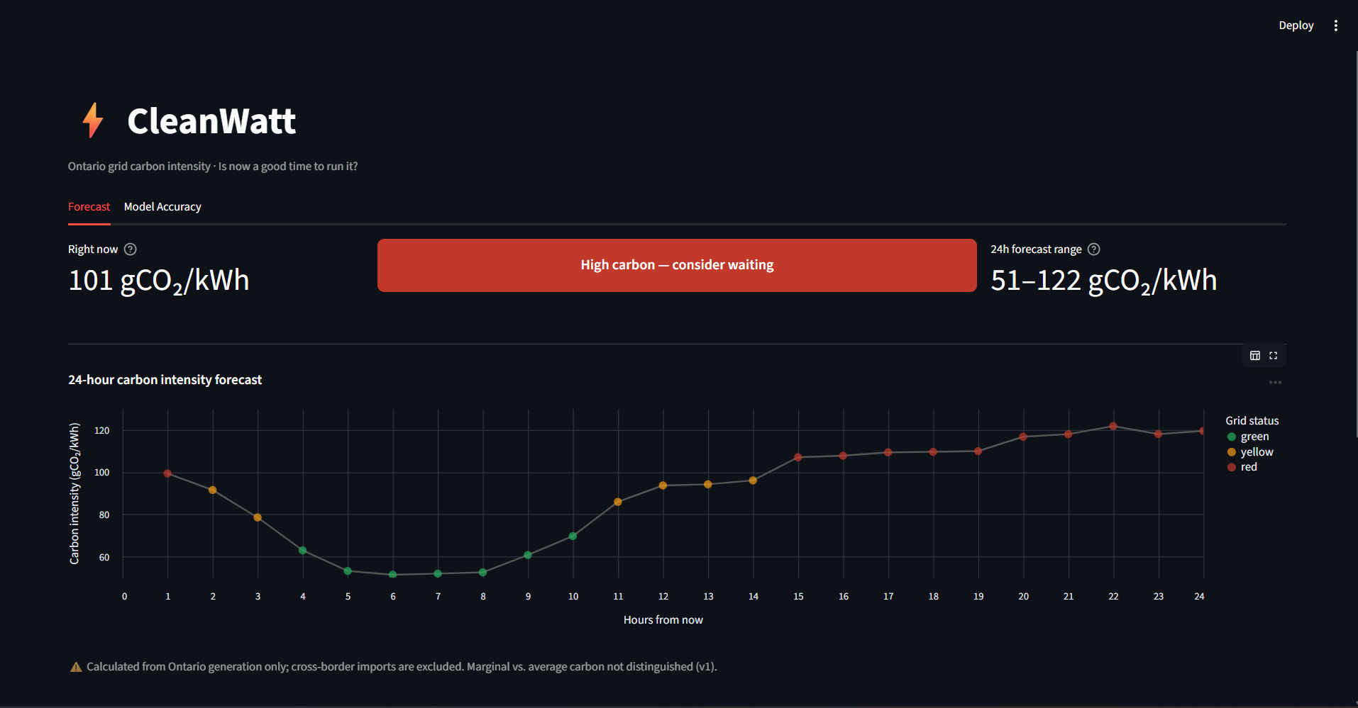
The Streamlit dashboard pulls live data from IESO and Open-Meteo at runtime, cached every 5 minutes. It shows a 24h forecast chart, a green/yellow/red intensity badge relative to today's range, and appliance window cards (Dryer 1h / Dishwasher 1.5h / EV overnight 6h / custom) that surface the lowest-carbon contiguous block for each appliance. A Model Accuracy tab plots rolling MAE and skill score over time. A GitHub Actions cron job appends daily predicted-vs-actual results to a forecast log and fires a drift alert when the rolling 7-day MAE exceeds 1.5× training MAE.

The hard part

The first version of the model used calendar features, carbon intensity lags, and the current fuel mix breakdown. Near-term forecasts (h=1–6) were solid, but skill scores collapsed past h=15 — barely above the "same hour yesterday" baseline. The problem is structural: the near-term signals (current fuel mix, recent lags) decay fast. At 18 hours out, the model had nothing to tell it what the grid would look like.

The fix was two new feature groups: IESO's own demand forecast, available hours ahead via their public reports, and Open-Meteo wind speed forecasts at 6h, 12h, and 24h leads. If demand is expected to spike tomorrow evening, or wind is forecast to drop, the model can now reason about that shift. Mean skill improved from +0.217 to +0.301, with the biggest gains exactly where the first version failed — h=18 went from +0.052 to +0.176, h=24 from +0.059 to +0.185. One odd pattern survives: skill still dips around h=15–16 before recovering at h=22–23, because at the 24h mark lag_24h is literally "carbon intensity right now" and the 24h wind lead lands precisely, giving the model a strong double signal at that pocket.

What I'm working on next

advisor.py was written to be UI-agnostic from day one — no Streamlit imports, plain Python functions in and out. The next step is a thin FastAPI wrapper around it for a mobile client: the core logic won't change, only the delivery layer. The GitHub Actions feedback loop is already logging predicted vs. actual daily, so drift detection is live; the mobile app will surface that signal directly to users.